Understanding the IP3 specification and linearity, part 1
In part one of this two-part story, the authors review the basics of intercept point specifications and linearity. For an expanded view of the equations, click here. Part two will discuss how to actually evaluate and interpret IPn.
For a variety of electronic devices ranging from RF mixers to low-noise amplifiers (LNAs), linearity is an essential performance attribute. The degree of linearity demonstrated by a component can make the difference between a successful device and a unit that fails to operate as designed. Intercept point (IP) specifications provide a useful tool for determining the degree of linearity exhibited by electronic devices.
IPn, which stands for intercept points of order n for some integer n≥2, consists of “virtual” parameters (i.e., the values are actually defined from other specifications). As a result, their values and extrapolations often remain vague. Admittedly, many electronic books or tutorials give some description of how IPn specifications are linked with input/output powers, power gain, and compression point. However, those reference works offer minimal, none, or incomplete explanations about IPn specifications and their origin.
Today, integrated functions such as an LNA, mixers, and a VCO (voltage controlled oscillator) can be built with the highest linearity (thus superior IP3) with advanced design techniques, and with proven RF processes. The design aim is to obtain the highest IP3 without sacrificing current consumption (bias circuit), gain, and size. Practically speaking, describing IPn orders up to 5, and eventually 7, can be significant. Today, however, the “order 3” (IP3) dominates when describing the normal operation of sensitive devices.
This article will use basic math and graphics to explain how IPn, and especially IP3, is generated and how its values are linked to essential quantities such as the input and output powers of a device. It will explain why high IP3 (thus, high linearity) is so important when evaluating performance. Finally, it will discuss some high-performance analog ICs in which linearity, high IP3, is a fundamental measurement of their good operation.
Why is linearity so important?
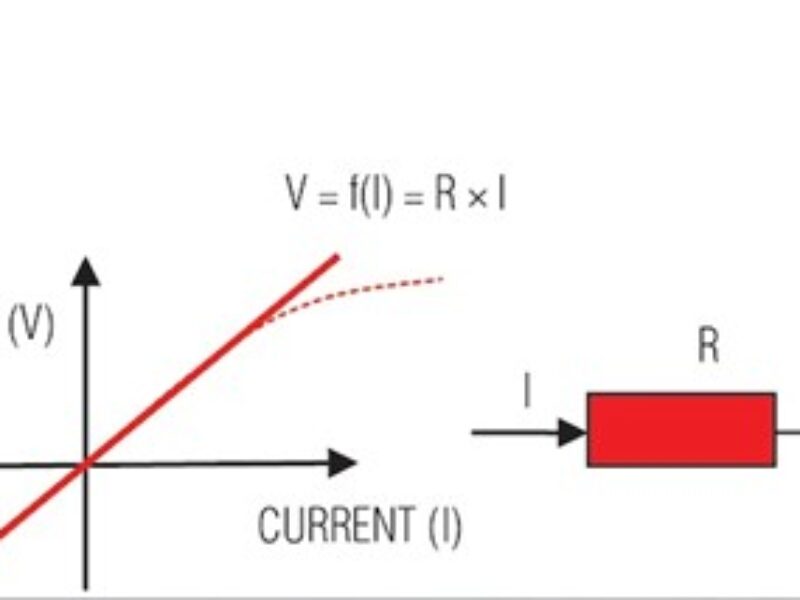
A principal objective for many electronic devices has been always to replicate simple, easy-to-reproduce, ideal mathematical functions. A simple illustration is the resistor which is designed to reproduce a linear relationship between voltage and current (VI). The resistor is simply the slope of the VI response.
We all know that the ideal relationship of V = R × I cannot be realized 100% of the time. One can approach it, but the inherent imperfections and limitations of the devices cause deviations in the ideal curve. This is particularly true when signals (I, V) are large and/or other conditions like temperature, humidity, and pressure vary. To compensate for these inherent deviations, we want the resistor, R, to be as linear as possible and remain so over wide ranges of signals and conditions. In reality, however, resistors have more complex curves in the (VI) characteristics (red dotted line in Figure 1).

Other IC components that require well-controlled linearity include amplifiers, data converters, VCOs, mixers, and PAs. With these ICs, deviations from the ideal VI relationship lead to instabilities, failure to meet specs, and interference. They can even cause malfunctions or destroy the device and/or entire system.
Measuring linearity
Depending on the class of signals and their dynamic ranges, different parameters and methods are defined to visualize, evaluate, measure, and compare the linear characteristic of an actual device.
Resistor linearity is typically measured in % of a nominal value of R. This is usually enough to appreciate the error that one introduces in current and voltage on the device.
The RF functions in an LNA, mixers, filters, PA, and other components can generate very large signal dynamics and introduce harmonics, interference, and saturation as critical effects of nonlinearities. Several parameters have been defined to characterize this nonideal relationship between input and output:
- 1dB compression point (CP-1dB)
- Compression dynamic range (CDR)
- Spurious-free dynamic range (SFDR)
- Desensitization dynamic range (DDR)
- Intercept points (IPn)
Since all the above terms indicate how good (or bad) the linearity of a device is, relations do exist between them. While this examination acknowledges the above class of parameters, it focuses exclusively on the intercept points, or how IPn (n) can be 2, 3, 4, etc. It will become clear that IPn (especially IP3) reveals the most about how nonlinearity negatively affects useful signals. It causes interference to be directly injected in the desired signal bandwidth. For this reason, one can focus here only on IP3 performance, regardless of the other parameters. Thus, in a few words, the higher the IPn, the more linear is the device.
Nonlinearity causes harmonics and intermodulation (IMn)
We begin by considering a general electronic function. Signals x and y are the input and output powers, respectively, and A is the transfer function between them (i.e., the “gain” if the device is an amplifier). Referring to the discussion of the resistor in Figure 1, in all real-world devices the curve is not a nice straight line indicating that “y is proportional to x.” Instead, the curve is not perfect and becomes distorted when signals are large.
When x and y are small, the curve is close to a straight line, but not 100% straight. Whether or not the designer realizes it, there are nonlinearities. When x and y are large, however, the nonlinearities are highly visible. In general, the device saturates; the output cannot respond correctly to any further increase in the input signal. This phenomenon is better illustrated by the -1dB compression point which shows the upper limit of the applicable signals (i.e., the dynamic range) (Figure 2).

Generally speaking, one can write:

Unfortunately (as you now know), this is never entirely so; the terms in x2, x3, x4 etc. are present as well. Their magnitudes depend on the strength of A2, A3, A4 etc., and they are responsible for the deviation of the transfer function A away from the desired, perfect, proportional law.
Assume now that we are in sinusoidal world where x(t) is a sinewave signal. Here x(t) contains only one frequency, ω. Therefore, by expressing it in a very general sinewave form:

We will focus only on the first term of the sum for the further discussions. (This simplifies the equation manipulations, since only the exponential effects will be used in our demonstrations.)
Let’s assume that the first term of the Euler form in x(t) is:

You see that y contains the same and unique frequency ω. We can draw an important conclusion from this: a perfect linear function or device will never generate any other frequency by itself.
There are two important observations to be made now:
x contains two frequencies: ωa and ωb.
It is easy to show that if the device is linear, it does not matter; y will reproduce exactly the same two original frequencies, ωa and ωb:

There are no other frequencies generated!
x contains multiple frequencies: ωa, ωb, ωc, ωd, ωn
Again, if the device is linear, the output remains a nice image with no distortion of x. The same original frequencies (no more and no less) are found in y. What happens when the device is not linear?
We start our analysis with x containing only one frequency, ω:

Thus, the device has generated multiple frequencies that were not present in the input signal, x.
The fundamental is the term y with ω; all the others, 2ω, 3ω, …i. ω,…n.ω (in fact, the integer multiple of ω) are called its harmonics. These harmonics are responsible for the signal distortion and noise.
At this stage, the situation is not that dramatic; the harmonics are (often) easy to filter out since their frequencies are relatively far from useful signals bands “glued” around the fundamental one (Figure 3).

The real annoying problem comes when you combine a nonlinear device and input signal containing several frequencies. This is especially troublesome when you have a perturbator close to the useful frequency. We will see what happens with two frequencies:

The term xa2 contains frequency 2.ωa, and the term xb2 contains frequency 2.ωb. The 2 above are the harmonics. Note now that strange effects are also appearing: arithmetic combinations of the originals. They are called intermodulation products (IM).
Finally, the term 2. xa xb contains frequencies ωa + ωb and Іωa – ωbІ. If the original frequencies are in a similar band, the four above terms will be situated relatively far away and, thus, easy to eliminate (even with inexpensive filters). The mixtures between the original frequencies, ωa + ωb, ωa– ωb, and ωb – ωa are also called second-order intermodulation products (IM2).
Third-order products: A3.x3
By developing (xa + xb)3, you will find xa3, xb3, 3xa2 xb, and 3xa xb2. Those will generate other intermodulation products with frequencies such as 3ωa, 3ωb, 2ωa + ωb, 2ωa – ωb, ωa+ 2ωb, and 2ωa – ωb. The mixtures between the original frequencies, 2ωa + ωb, 2ωa – ωb, and 2ωb – ωa, are also called third-order intermodulation products (IM3).
While the terms 3ωa, 3ωb, 2ωa + ωb , and ωa+2ωb are easy to eliminate, this is no longer true with some IM3 terms like 2ωa – ωb and 2ωb – ωa that are in the same frequency range as ωa and ωb. If one of these latter terms carries information (modulated), then you must be sure that the other terms will not interfere with the intermodulation terms. As we said earlier, they fall in the same bands as the useful signal bands and thus cause unrecoverable jamming and interferences.
Figure 4 shows that even with strong expensive filters, it will not be easy (even impossible) to remove the IM3 terms because they are embedded in the useful band! This is precisely why in RF the third-order terms are so critical and must be known, measured, and minimized everywhere in the signal chain.

Fourth-order products: A4.x4
A similar pattern also applies to frequencies 4ωa, 4ωb , 2ωa + 2ωb , 2ωa – 2ωb, ωa + 3ωb , 3ωa + ωb, 3ωb – ωa, and 3ωa – ωb. As with the second-order terms, all the frequencies here are quite removed from the 2 fundamentals. From these observations, we can easily see that IM products are more dangerous with an odd order of n (i.e., IP3, IP5, IP7, etc.).
Nth-Order Products: An.xn
The same process can be applied to the term (xa + xb)n. Hopefully, for practical devices, the higher-order terms vanish rapidly and can be neglected (this is usually true above IM7 and even sometimes with IM5).
We could continue the discussion by considering x with more than two frequencies, ωa, ωb, and ωc. However, that effort would not add much to our understanding since they will simply give us more IM2, IM3, IM4, etc. frequencies.
Part two of this story will discuss how to actually evaluate and interpret IPn.
 If you enjoyed this article, you will like the following ones: don't miss them by subscribing to :